
We explained in our book “Remote Sensing and GIS for Ecologists – Using Open Source Software” among other change detection methods also the change vector analysis practically using the rasterCVA() command in the RStoolbox package, as well as outlined the approach graphically. During my last lecture on temporal and spatial remote sensing approaches I realized that the graphic needs some fixing as well as the RStoolbox function, moreover, certain explanations were missing. Hence, Benjamin Leutner adapted the rasterCVA() command and I tested it again and created new graphics explaining this approach for land cover change analysis.
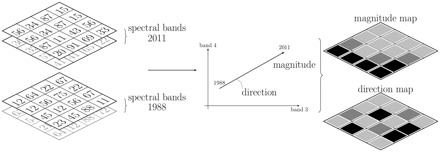
general Change Vector analysis explained. Graphic from the book “Remote Sensing and GIS for Ecologists“
The first graph that is also in our book shows the general approach. Two bands for each year (e.g. the RED and NIR band, but also the Tassled Cap output can be used) are taken and the changes in pixel values between these two years are shown as angle and magnitude.
We realized some things were missing: first the explanation what the angle actually means and second a link of actual results and the xy-graph.
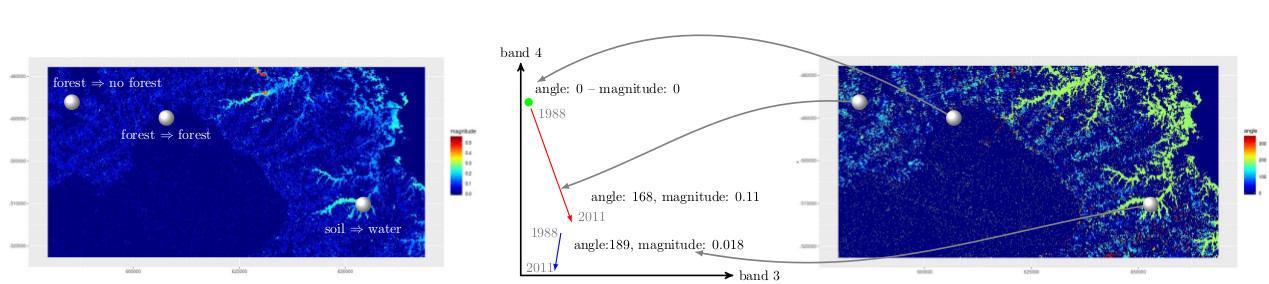
Change Vector analysis explained on three change classes using the actual rasterCVA() output and band values.
In these new figures we show the actual results of the land cover change vector analysis using band 3 and 4 of Landsat (E)TM for the study region used in our book and three angles and magnitudes of pixels values between 1988 and 2011.
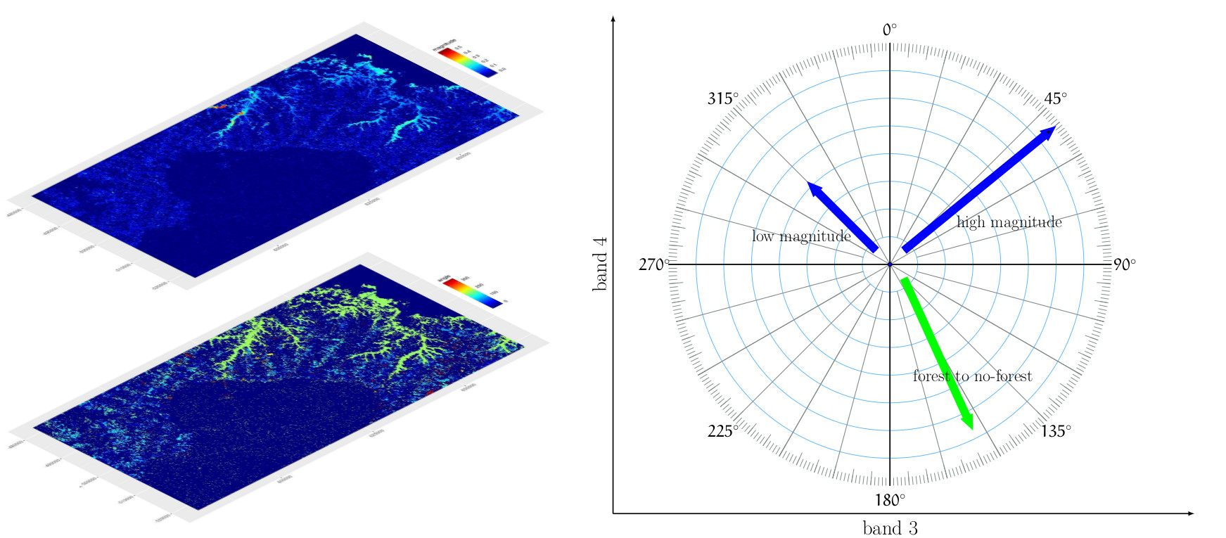
Meaning of angle and magnitude values from rasterCVA() analysis in RStoolbox
In the second image we outline the meaning of the angle provided by rasterCVA() as well as the magnitude which is the euclidean distance of the pixel values between 1988 and 2011.
Please approach us if you have any suggestion how to improve it or if we introduced any errors.
Please update to the newest development version to access the updated RStoolbox functionality!